Activity 17 - Photometric Stereo

Light striking an object at a certain direction would get reflected a specific orientation. Detecting this reflected light would only mean capturing one component of the intensity. This means that illuminating an object in different positions results to different shadings in the images of the object. Photometric stereo is a technique of using these different shading information for 3D reconstruction.

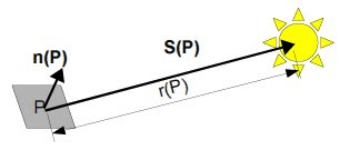
In this activity, it is assumed that the light striking the object are uniform plane waves. From the figure above, the direction S(P) is now a constant for all points P on the object. This allows a simple calculation of this direction, which is just proportional to the location of the light source with respect to the object:

(each row represents the 3D coordinates of one light source with the object as origin)


(k is the proportionality constant)

Intuitively, the brightness of a point P on the object would be given by the equation

where ρ(P) represents the reflectivity of that point, ň(P) is the normal vector at point P and S0 is the vector from the point to the source, which is now considered a constant for all points on the object due to the plane wave illumination. The intensity detected is proportional to this brightness by the same proportionality constant k in the equation for V:

We can set:

so that from a set of images of the object using N different light source locations:

we can calculate by matrix operations:

Upon knowing g, the surface normal vectors of the object can be calculated:

From the surface normals, the 3D object can be reconstructed since the gradient of the object surface is equal to the surface normal vectors. It can easily be shown that from 3D coordinates of the object

the gradient can be calculated to obtain the relations:

The reconstruction can be completed from the surface normals by calculating the z using

In this activity, four images are obtained using four different light sources, as shown below, with the corresponding light source locations. (Note: The images shown below are normalized individually).

Image 1 (V1 = {0.085832, 0.17365, 0.98106})

Image 2 (V2 = {0.085832, -0.17365, 0.98106})

Image 3 (V3 = {0.17365, 0, 0.98481})

Image 4 (V4 = {0.16318, -0.34202, 0.92542})

Applying photometric stereo described above, the shape of the object was reconstructed and the result is shown below. The surface of the reconstruction is not very smooth. However, the shape is still defined.

3D reconstruction of the object

I would like to give myself a grade of 10 for successfully implementing photometric stereo for the given images.
I acknowledge the help of Mr. Orly Tarun and Mr. Mark Jayson Villangca and the guidance of Dr. Gay Jane Perez in doing this activity.

Activity 13 - Correcting Geometric Distortions

In imaging, light rays from a point on an object is captured by camera lenses, refracted and focused onto the recording plane of the camera, whether on a film or a CCD. However, due to the shape of the lenses, light rays from a single object point does not focus on a single point on the recording plane. This is due to the fact that light rays refracting at the edge of spherical lenses (marginal rays) behave differently than those close to the center or the optic axis of the lens (paraxial rays). For the same reason, parts of the object directly 'passing' through the edge of the lenses upon imaging would result to some geometric distortions. The two most common are the pincushion and barrel distortion, which produce images shaped like a pincushion and a barrel, respectively.

In metrology, it is critical to obtain highly accurate data from images. In this regard, distortions are undesirable, causing errors in the measurements. In this activity, a method for correcting geometric distortions is presented.

The main idea behind the reconstruction is to image a regularly occurring pattern, such as a grid or a checkerboard. From the imaged pattern, coordinates upon distortion for each point on the ideal pattern are known and can provide the necessary information for obtaining the distorting function (see image below).

Ideal grid (right) and distorted grid (left) with
corresponding vertex points specified by the arrow
(image taken from [1]).

Other points on the ideal image can then be mapped on the distorted image using the same transformation as the vertices. Using the four vertices of a square in the pattern, a relation can be obtained regarding the transformation in the coordinates of the distorted grid:

The same transformation relation can be used for the points inside the square. To obtain this relation, matrix operations are used to calculate for the coefficients, C:

These coefficients is used to calculate for all the points inside the square:

Grayscale or RGB values of the ideal image can then be obtained from the corresponding values on the distorted image upon knowing points of the distorted image corresponding to the ideal image. Since images are indexed in pixel coordinates, only integer values are accessed for the distorted image. Different algorithms can be used to determine the grayscale or RGB value for cases when non-integer valued coordinates on the distorted image is calculated. One is the nearest neighbor algorithm, which basically takes the value of the distorted image at the nearest integer coordinate of the calculated distorted coordinates. Another algorithm, bilinear interpolation, interpolates the value using the four nearest neighbor pixels of the calculated distorted coordinates. Using the equation:

the grayscale or RGB value v(x,y) is obtained following similar matrix operations for obtaining the distorted coordinates. The four nearest neighbor pixel values are used in the same way as the four vertices of the square, for calculating the coefficients a, b, c, and d. The pixel value for distorted coordinate is then obtained and set as value on the ideal image to complete the reconstruction.
The method described above can also be used to correct other types of distortion since the distorted image is mapped to an ideal grid with a specific transformation. This transformation can be of different type to correct for different distortions.

Two trials were made for correcting of the image below. For analysis, reconstruction using vertices of the squares of the grid overlaying the image (Trial 1) was compared one using vertices of the square composed of the four basic squares in the image (Trial 2).

Distorted image
(original image taken from http://www.karbosguide.com/books/photobook/chapter34.htm)

Coordinates of the vertices were obtained using locate() in Scilab. Then the ideal grid was constructed by selecting the coordinates of the square with (approximately) no distortions, and building up all the other squares in the ideal image. The undistorted square used for Trial 2 is the square composed of the four central squares in the image specified by the four red dots. For Trial 1, only the upper left square in the four central squares was used.
Using the vertices of the squares in the distorted and ideal grid, the coefficients were obtained to determine distorted coordinates for all the points inside the square. Nearest neighbor and bilinear interpolation algorithms were then applied to obtain the RGB values of the ideal image. The results of the reconstructions are shown below (the whole image was not reconstructed).

***Click on the image below for a larger image

Trial 1

Nearest-neighbor and Bilinear interpolation

Trial 2

As demonstrated in the results, the bilinear interpolation algorithm provides a better reconstruction compared to the nearest-neighbor for both trials. The bilinear interpolation gives a more accurate RGB value. This is better shown in the lines of the grid. The nearest-neighbor algorithm has lines that are more jagged.
In comparing the two trials, it seems logical that using the small squares should result to a better reconstruction. Zooming in on one part of the image, this is shown more evidently (shown below, for the bilinear interpolation images). The reconstruction for Trial 1 is much smoother compared to Trial 2, which contains more artifacts. The reason for this is because the small squares would provide a more specific set of coefficients for calculation of distorted grid coordinates in an area. However, as noticed in the images above, the reconstructions for Trial 1 are actually rectangular, while for Trial 2, the images are square. The obtained undistorted central square for Trial 1 is not a square, not like the square obtained for Trial 2. As noticed, the square used in Trial 1 is not directly at the center, while for Trial 2, it is exactly at the center. The approximation that the square chosen is undistorted may not be valid for Trial 1. For Trial 2, since the square is directly at the center, there would be no offset on whether the square is perfectly undistorted.

Trial

1 2

In this activity, I would like to give myself a grade of 10 for producing a very good correction of an image with relatively large distortion. Moreover, I also examined the use of smaller squares compared to larger squares in the reconstruction (Trial 1 and 2).
I would like to thanks Ms. Winsome Chloe Rara and Mr. Mark Jayson Villangca for their help in doing this activity. I also acknowledge Dr. Maricor Soriano for her discussions regarding this activity.

Reference
[1] M. Soriano, Applied Physics 186 Activity 13 Correcting Geometric Distortions Manual, 2009.

Activity 16 - Neural Networks

As mentioned in Activity 14, object classification is one human capability that is commonly investigated and modeled for implementation in computer vision. It is actually a process of the human brain analyzing the information detected by the senses to classify objects. Inside the human brain are networks of neurons working together to process the information.

Neural networks are standard algorithms that have been used to model this process inside the brain. Similar to how the mind works, the basic concept of the algorithm is it first 'learns' what a class is from the features of objects that is known to belong in that class. Once the feature pattern for a class is known, classifying objects is straightforward by recognizing the class pattern in the object features observed.
The critical part in neural networks is the learning process, which is also crucial for human beings. Learning in neural networks is by basically determining the weights given to observed features. The network can be modeled by a connection of layers of nodes - input, hidden and output. Features from visual information are fed to input nodes which then pass a new weighted information to the hidden layer or layers. The hidden layer directs the information to the output node to combine the information into an outcome which determines the classification of the object. If object features from known classes are set as input, the network can calculate the error of its output. An iterative process then proceeds to readjust the weights applied to the input information in the connections of the nodes to minimize the error of the output. Certain parameters can be used in the iteration such as the learning rate of the network and the time set for the network to learn (which can be described as how much iteration is needed). Once the target output (or close to the target) is obtained, the final weights can be used in the network to classify unknown objects.
The ANN (Artificial Neural Network) toolbox for Scilab was applied in this activity for classifying normal or crenated RBCs. Training set and test set features from the previous two activities were used. A neural network was initialized with 2 input nodes (for the 2 basic features of an object) , 2 hidden layer nodes, and an output node with output values specifying whether crenated (1) or normal (0). The training set features were used for the learning process, and the weights obtained was then applied to classify the test set.
First, the effect of learning rate and training cycles to the output of the learning process was examined. The mean output value for the 5 input crenated RBC training set was plotted with respect to both the learning rate and training cycles. The 3D plot shown below signifies that increasing the learning rate would result to a faster approach of the training result to the target output even though there is a limited number of training cycles. On the other hand, for a low learning rate, increasing the training cycles will produce results approaching the target output. On both cases, further increase on learning rate and training cycle result to minimal improvement. The results seem logical because a higher learning rate would result to faster convergence to the desired weights, while more cycles would mean training the network at a longer time, making it more accurate. This also means that the high learning rates and low training cycles would results to faster training for the network, which was observed in the simulations. However, for a high learning rate, the weights would change more inaccurately producing a final output of weights that are less reliable compared to lower learning rates. This was verified because trained networks with high learning rates result to a lower percentage of correctly classified RBCs as compared to low learning rates. As a consequence, the training parameters used was 0.1 learning rate and 10000 training cycles. The resulting network was used to classify the test set of RBCs.

3D Plot of neural network training output for crenated RBC vs
learning rate and training cycle

Trial 1


Trial 2

Table of classification results using a network trained
at learning rate = 0.1 and training cycles = 10000

The artificial neural network classification provided the same accuracy as the linear discriminant analysis presented in the previous activity. This shows a successful implementation of neural networks for pattern recognition and classification. By improving the data to be processed as mentioned in the Activity 14, a more accurate or maybe even perfect classification can be attained. This shows that neural networks can be a good descriptive model of how the human brain works, which would can be a powerful tool in computer vision and robotics. This would also have significant impact for the usage of technology in institutions such as hospitals and schools for academic and research purposes.
I would like to give myself a grade of 10 (and possible bonus for additional analysis) for successfully implementing neural networks for the classification of normal and crenated RBCs.
I would like to thank Dr. Gay Jane Perez for the discussions regarding this activity and to Mr. Cole Fabros for his blog regarding the use of ANN toolbox in Scilab.

Activity 15 - Probabilistic Classification

From the previous activity, red blood cells (RBCs) are classified as normal or crenated by using visual information obtained by image processing as basic features that are the basis for discriminating the normal from the crenated RBCs. More specifically, minimum distance classification was used in classification by basically determining to which mean set of features (either for normal or for crenated) the object feature set to be classified is closest to.

In this activity, a different technique called linear discriminant analysis (LDA) is applied for classifying object features by minimizing the error in the classification of the objects. Linear discriminant analysis is based on conditional probability such that from the occurence of a given set of measurements, there is a probability for one object, for example, to be normal or crenated. Determining this probability is not direct. But it has already been shown [1] that this can be related to the conditional probability that an object or set of objects is known to be one class or the other (in this case normal or crenated), a set of measurements are taken for that class. More specifically, the classification is done based on the formula below:

where μi is the mean feature set for the class i, C is the pooled covariance matrix*, both obtained from the training set, xk is the test object feature set to be classified, and pi is the prior probability of that class**. The quantity fi represents the probability that the given set of features of a test object belongs to class i. This suggests that the larger fi means it belongs to that class. For example, if the calculated f for normal is larger than that calculated for the crenated, then, the object is classified as normal. Otherwise, it is crenated.

*pooled covariance matrix - weighted sum of the covariance matrix of the set of features of the object in class for all classes with weights depending on the number of objects in that class over the total number of objects in the test training set
**prior probability - assumed as the number of objects in that class in the training set over the total number of objects in the training set

Using the training set features and the test set features obtained from the previous activity, linear discriminant analysis is applied.

From the results presented in the table above, the improvement in the classification was only observed for trial 2. More specifically, the improvement was in the classification of the crenated RBCs. From the scatter plot of the object features, the crenated RBCs in trial 2 are very close to the region of the normal RBCs. LDA was able to discriminate more crenated RBCs in this region, however, only improving the classification by approximately 2%. Actually, the 2% increase represents only one additional correctly classified crenated RBC. There are no more improvements obtained for trial 1 and the classification of normal RBCs in trial 2 because minimum distance classification was already sufficient. The features correctly classified have probabilities that are already reflected in their distances from the mean for normal and crenated RBCs. Still, LDA can be used as a more stringent classifier as compared to the minimum distance classification.
In this activity, I would like to give myself a grade of 10 for successfully implementing LDA to the data obtained from the previous activity. I was also able to somehow discuss the process and show the advantage of LDA.
I would like to thank Dr. Gay Jane Perez for guiding is in this activity, and to Ms. Jica Monsanto for some discussions.

Reference
[1] http://people.revoledu.com/kardi/tutorial/LDA/LDA.html#LDA
[2] http://en.wikipedia.org/wiki/Conditional_probability

Activity 14 - Pattern Recognition

Classifying objects accurately based on visual information is one of the most basic yet interesting and amazing representation of how the human brain and the human senses work together. Characterization of objects usually starts with identifying the kinds or classes of objects. This can be done by first defining the basic features of the objects in a class, usually by shape, size or color, that can be used to easily discriminate objects among different classes. The human brain stores this knowledge of features of objects in a class and also determining the main differences in the basic features among classes. Using this information, new objects can be classified based on the basic features compared with that defined for the classes, finding out to which class its set of features most closely resembles.

This is the model used by computer vision for automatically classifying objects based on visual information. The process revolves around pattern recognition by creating the set of basic features for an object to serve as pattern. Image processing techniques can be applied to provide the automated gathering of basic feature sets. Classes are defined by the patterns of objects belonging to that class. Then, new objects, having features to be classified are determined on which class they fall into.
Minimum distance classification is one way of quantifying the resemblance of a pattern of an unclassified object to the patterns of different classes of objects. The principle basically follows the fact that the object can be classified to a class to which its set of features has the least distance from the mean of the features of the objects from that class. By having the set of features contained in a feature vector (each element represents a feature and each vector represents an object), the distance can be calculated using the Euclidean distance formula.
In this activity, red blood cells (RBCs) are classified whether normal (Erythrocyte) or crenated (Echinocyte). Crenation happens when a cell is exposed to a hypertonic solution, causing it to lose water by osmosis and shrink producing an abnormally shaped cell (http://en.wikipedia.org/wiki/Crenation). An image of a normal and crenated RBC is shown below (indicated by the arrow).

Normal


Crenated
(image taken from http://www.healthsystem.virginia.edu/internet/hematology/hessidb/alphabeticalglossary.cfm)

It is important to study the effects of the environment to a cell or to an individual whether it can survive in it or not. Analysis of RBCs in different solutions with different concentrations is one way of providing this study. Classifying normal and crenated RBCs and providing a statistics for the classified objects is therefore critical. However, sufficient number of samples may be required to make conclusions about the cell-environment interaction. Classifying a large number of RBCs for a sufficient sample size is a very tedious and time consuming task, which is why automation by computer vision has been a rapidly-developing technology. Automatic recognition of crenated and normal RBCs is demonstrated here.
Based on the change in shape of the crenated from normal RBC, a set of basic features can be created. Thresholding (im2bw()) was applied first to separate the cells in the image from the background. Labeling (bwlabel()) was then applied to clean the image from small fragments and incomplete cells (at the edges) and also to remove overlapping cells. Morphological operations should not be applied to remove these since this may alter the shape of the cells, which is critical in defining the features. Two trials were done using images with both normal and crenated RBCs as shown below.

Trial 1

Original

(image taken from http://www.healthsystem.virginia.edu/internet/hematology/hessidb/alphabeticalglossary.cfm)

Thresholding


Labeling

Trial 2

Original
(image taken from http://www.isrvma.org/article/63_1_1.htm)

Thresholding


Labeling

From the results of image processing, five normal and five crenated RBCs were visually classified and taken to serve as the training set and to define the set of basic features for the corresponding class. The basic features chosen were (i) the ratio of the square of the perimeter versus the area, and (ii) the ratio of the standard deviation of the radius of cell versus the mean. These features were used so as to highlight the main difference in the shape of the normal and crenated RBCs. Also, dimensionless units should be used for the method to be invariant in terms of size.
The features were easily obtained by using the command follow() in Scilab to determine the coordinates of the contour of the cells. The perimeter is just the number of the coordinates of the contour, while the area is obtained using Green's theorem (Activity 2). The standard deviation of the cell is obtained from the coordinates of the contour by first subtracting the mean (x, y) to the (x, y) values of the contour. The set of radius was then obtained by Pythagorean formula using the resulting (x, y), and then calculating for the standard deviation. The mean of the set of features for the five objects would define the features for corresponding class.
Now, for each cell, the set of features was extracted to serve as the test set as described previously, and this was compared to the mean for the normal and the mean for the crenated RBCs. By minimum distance classification, if the set of features for that cell is closer to the mean for the normal RBCs, then it is classified as normal. Otherwise, it is crenated. The resulting classification was verified by comparison with visual classification.
Analysis was also done by looking at the scatter plot of the object features, shown below. This would determine if the features for a class are well separated from the other class. The training set features indeed are isolated from each other. However, the test set still has some of the cells 'creeping' into the region of the other class. There is a large deviation of the features for the crenated RBCs, as seen in the plots, more obviously in trial 2. However, it can still be noticed that there is a definite region to where most of the objects in a class fall into.

Trial 1

Trial 2

From the minimum distance classification, the summary of the classification is presented in the table below. Based on the scatter plot, the results seem logical because for trial 1, the normal and crenated features have a more definite separation compared to trial 2. Moreover, the features for the crenated RBCs have a higher deviation from the mean compared to the normal and many crenated RBCs are very close to the normal RBC features. This produced a very low correctly classified percentage of the crenated RBCs. Since the normal RBCs are very close to the mean, it has a very high classification percentage. One major reason why there are better results for trial 1 is because the image has a higher resolution compared to that used for trial 2. The cells occupy more pixels, which helps in increasing the effect of the difference in shape from the normal and crenated RBCs. Low resolution images are difficult to handle for the classification process. The 'spikes' at the edge of the crenated RBCs would no longer be evident if it is represented by fewer pixels.

From the results obtained, this technique demonstrates a feasible method for computer vision in classifying RBCs. After initializing the process by taking known crenated and normal RBCs for the mean set of features, automatic classification can be applied to classify RBCs, for example, in a whole slide, or for different slides, using the same setup (magnificatio, camera saturation, etc.). Some of the limitations are (i) the mean set of features can only be used in the same setup, (ii) overlapping cells are not classified, and (iii) high resolution setups are needed for accurate cell classification.
For this activity, I would like to give myself a grade of 10 for doing a very good job. I used a very interesting sample and I think my classification is very satisfactory for this kind of sample. The discussions I provided are, somehow, also extensive.
I would like to thank our professor, Dr. Gay Jane Perez, for the guidance in doing this activity, and Ms. Jica Monsanto and Mr. Jay Samuel Combinido for their help in the process of determining features for classification.

Reference
M. Soriano, Applied Physics 186 Activity 14 - Pattern Recognition Manual, 2008.