Activity 6 - Properties of the 2D Fourier Transform

annulus

square

square annulus

double slit

two dots

Pattern (left) and corresponding 2D Fourier transform (right)

Some patterns were generated using Scilab and the corresponding (2D) Fourier transforms are shown above. (Patterns are symmetric).
Code for generating patterns:
Annulus:
x = [-64:1:64];
[X,Y] = meshgrid(x);
r = sqrt(X.^2 + Y.^2);
annulus = zeros(size(X,1), size(X,2));
annulus(find (r <=32)) = 1.0; annulus(find(r<=16)) = 0.0; Square: sq = zeros(129, 129); temp = ones(33, 33); sq(49:81, 49:81) = temp; Square Annulus: sqannulus = sq; temp2 = zeros(17, 17); sqannulus(57:73, 57:73) = temp2; Double Slit: slit = zeros(129, 129); slit(:, 55) = 1.0; slit(:, 75) = 1.0; Two Dots: dot = zeros(129, 129); dot( 65, 55) = 1.0; dot( 65, 75) = 1.0;
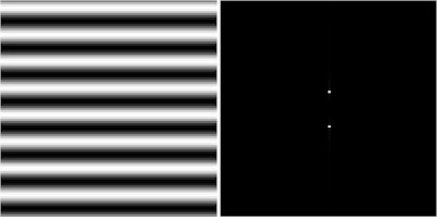
In this activity, the anamorphic property of the Fourier transform is analyzed. First, a 2D sinusoid (similar to a corrugated roof) is created. To examine the spatial frequencies of this image, the Fourier transform was obtained. Furthermore, the frequency of the sinusoid was varied (f = 4, 8 and 16). The results are shown below.

f = 4

f = 8

f=16
2D sinusoids (left) with the specified frequencies
and their corresponding Fourier transforms (right)

As noticed in the Fourier transform of the images, the peak values on the 2D-fft is moves farther along the axis perpendicular to the sinusoid lines as the frequency of the sinusoids are increased. This demonstrates that the Fourier transformation shows the spatial frequencies of an image. The sinusoids have frequencies along the vertical and it is presented in the same axis in the Fourier transforms.
Scilab code for generating 2D sinusoids and displaying the Fourier transforms (modulus):
nx = 100; ny = 100;
x = linspace(-1,1,nx);
y = linspace(-1,1,ny);
[X,Y] = ndgrid(x,y);
f = 4 ; //for varying frequency
sinusoid = sin(2*%pi*f*X); //the 2D sinusoid
fft_sinusoid = fft2(z); //obtain Fourier transform
imshow(abs(fftshift(fft_sinusoid)),[]); //display modulus of the transform

Notice, however, from the code above that the sinusoids generated have negative values (based on the sin() function of Scilab). Of course, this is not realistic because standard images taken are non-negative. One way to simulate this is by adding a constant bias to the sinusoids such that there are no negative values. This would shift the sinusoids and, as if, they are riding on a DC signal. Again, taking the Fourier transform, the obtained result is shown below.
(As a comparison, the unbiased (left) and its Fourier transform (bottom) is placed side by side with the biased (right) and its corresponding transform. Notice that the unbiased and biased 2D sinusoids are identical. This is the limitation of the imshow and imwrite functions because it requires normalized images, and therefore, also altering the information contained in the images because no negative values can be shown or written as an image.)

2D sinusoids without (left) and with (right) bias

Fourier transforms of the unbiased (left) and biased (right).

The resulting Fourier transform of the sinusoid with a constant bias shows a central maximum. The reason for this is because the aside from the sinusoid signal, there is also a DC signal which is the constant bias as an additive term. The frequency of a DC signal is actually zero which accounts for the central maximum.

As a consequence of non-negative values in the images, capturing interferograms (such as the result of a Young's Double Slit Experiment) would result also to a sinusoid but from positive minimum (can be zero) and maximum values. This is similar to a sinusoid with a constant bias. To determine the actual frequencies of the results, data can ,initially, be subtracted by the average of the minimum and maximum values. This would make the sinusoid oscillate symmetrically about zero and, in turn, a pure sinusoid signal is observed. Then, Fourier transform can be applied to obtain the actual frequencies of the interferogram.
If a non-constant bias is added it would be hard to determine the adjustment needed. However, for example, if low-frequency sinusoids are added to the interferogram, it can simply be subtracted from the Fourier transform. The center of the transform of the 2D image represents the low frequencies, and this can simply be removed. If the frequency of the unwanted signals added are known, it is much easier because it can easily just be subtracted. But for example, for noise, which is of unknown frequency, it is difficult. Usually, these are of low frequencies so the previous suggestion might work.

2D rotated sinusoid (left) and the corresponding Fourier transform (right)

Scilab code to generate rotated sinusoid:
nx = 100; ny = 100;
x = linspace(-1,1,nx);
y = linspace(-1,1,ny);
[X,Y] = ndgrid(x,y);
f = 4; //frequency of sinusoid
theta = 30; //angle of rotation in radians (+ for counterclockwise)
z = sin(2*%pi*f*(Y*sin(theta) + X*cos(theta))); //generate rotated sinusoid

Further analysis was done in the Fourier transform of a sinusoid. This time, first rotating the sinusoid and then, taking the transform. As can be seen from the figure above, the axis of the sinusoid was rotated. As a consequence, the axis of the Fourier transform (in frequency space) is also rotated. The result demonstrates the property of the Fourier transform for obtaining the spatial frequencies in an image. Because the sinusoid is along a rotated axis, the spatial frequencies (which is actually the frequency of a component sinusoid of an image) would be along the same rotated axis.

It is also interesting to look at a combination (multiplication) of different sinusoids in X and Y. An easier way to visualize this is by providing a combination of different sinusoids in succession as presented below.

Sinusoid in X (left) with f = 4, and the corresponding Fourier transform (right)

Sinusoid in Y (left) with f = 4, and the corresponding Fourier transform (right)

Combination of the two previous sinusoid (left), and the corresponding Fourier transform (right)

Combination of the previous sinusoid with a sinusoid in X with f = 8 (left)
and the corresponding Fourier transform (right)

Combination of the previous sinusoid with a sinusoid in Y with f = 8 (left)
and the corresponding Fourier transform (right)

Notice that upon combining the sinusoids, the Fourier transform of the result looks like a spread of one of the Fourier transform to the Fourier transform of the other sinusoid in the combination. This is what basically happens in convolution. Now, it is known (also from previous activities) that the Fourier transform of the convolution of two functions can be obtained by multiplying the Fourier transforms of the two functions. The reverse is seen here. Initially, there is a multiplication of two images or sinusoid functions (combination of two sinusoids). The Fourier transform of the combination can be obtained by convolving the Fourier transforms of the two images or functions.

Scilab code for generating the combination of sinusoids in X and Y:
nx = 100; ny = 100;
x = linspace(-1,1,nx);
y = linspace(-1,1,ny);
[X,Y] = ndgrid(x,y);

z = sin(2*%pi*4*X); //sinusoid in X with f = 4
z1 = sin(2*%pi*4*Y); //sinusoid in Y with f = 4
z2 =sin(2*%pi*4*X).* sin(2*%pi*4*Y); //combination of sinusoid in X and Y with f = 4.
//z and z1 are simply multiply element by element

z3 = z2.*sin(2*%pi*8*X); //combination of sinusoid in X and Y with f =4 and sinusoid in X with f =8.

z4 = z3.*sin(2*%pi*8*Y); //combination of sinusoid in X and Y with f =4 and sinusoid in X and Y with f =8.

One important property of Fourier transform is linearity. This can be demonstrated by having an image that is a sum of different sinusoid signals. Intuitively, a linear transformation acting on a sum can be distributed into a sum of the transforms of each added terms. So for example, if the combination of X and Y sinusoids is added with a rotated sinusoid (X sinusoid rotated by 30 radians), the transform of the sum is basically the sum of the transform of the X and Y sinusoids and the transform of the rotated sinusoid. Indeed, this is verified by the results below.

Combination of sinusoids in X and Y with f = 4 (left)
and the corresponding Fourier transform (right)

Rotated sinusoid in X (angle of rotation = 30 radians) with f = 4 (left)
and the corresponding Fourier transform (right)

Sum of the two previous sinusoid function images (left)
and the corresponding Fourier transform (right).
The transform, indeed, looks like the addition of the Fourier transform of the two previous sinusoid function images.

For this activity, I would like to give myself a grade of 10 for a job well done (and ahead of time).
I would also like to acknowledge Winsome Chloe Rara for her help in doing this activity and the guidance of our professor Dr. Maricor Soriano.

Activity 5 - Fourier Transform Model of Image Formation

Fourier transform is a linear transformation that results into a representation of a data or object in the inverse of its dimensions. In the case of an image, it generates the spatial frequencies of the figures in the image. The lens actually acts a Fourier transformer of the object or light that it collects and focuses. Using the functions in Scilab (fft2, fftshift and imcorrcoef (convolution)), it is easy to demonstrate the Fourier transform process.
***Please click on the images to enlarge and have a better visual.


Similar to this circular light going through a lens, the image on the focus of the lens is similar to the Fourier transform shown. This resembles the analytical Fourier transform of a circle. Basically, the Fourier transform of the circle can be reconstructed back to the image of a circle. From the inverse space of the Fourier transform, taking the Fourier transform of the inverse space results in the inverse of the inverse space, which is actually the dimension of the original image.

However, using the A-shape, notice that there is an inversion upon applying the the fft2 twice. This was not observed for the circle because it is symmetric. The reason for this can be traced to the analytical form of the Fourier transform. The operation of two forward Fourier transforms is not the same as the operation of a forward and then an inverse Fourier transform, which would result in the same orientation of the original function. What results in the analytical form for a function f(x) upon applying the two forward Fourier transforms is in the form f(-x) (with some factor). It translates to the image being inverted.

Since the Fourier transform is linear, it can also be applied into other operations that have important applications. One is the convolution of two functions. It determines the spreading effect of a certain function on another function. Similar to imaging systems, the optical system used for imaging has a certain function that spreads the function defined by the object resulting in an image that is not exactly the same as the object. Although convolution is a complicated operation, a direct multiplication of the Fourier transforms of the functions in the convolution can actually be done to obtain the transform of the convolution.

Using the Fourier transform as the lens, the circle image can act as the aperture of this simulated imaging system. The multiplication of the Fourier transform of the object and the circle image results to the transform of the convolution. Taking the inverse Fourier, the convolution of the image with the transfer function of the optical system is obtained. Again, there is inversion of the image due to the application of two forward Fourier transforms, instead of one being an inverse. Notice that for larger apertures, a more accurate image of the original object is formed. This demonstrates that finite lens apertures cannot capture all light coming from the object, and therefore, making the reconstruction of the image imperfect.

Another process related to convolution and the Fourier transform is correlation. In comparison with convolution, it is also a linear process which can involve simplification (by multiplication) upon using Fourier transforms (and conjugate of one transform) of the correlated functions. The correlation basically takes the “degree of similarity” between two functions. As a consequence, it has been of great value for use in “template matching, pattern recognition and edge detection.”

As seen in the figure above, the pattern or template ‘A’ is correlated with the statement image. As a result, high correlation values occur at the corresponding location of the statement image with the letters A. This demonstrates correlation for template matching or pattern recognition.

For demonstration of edge detection, the patterns shown above are convolved with the ‘VIP’ image presented previously. The resulting correlation (using imcorrcoef) illustrates a highlight on the parts of the image with the same orientation as that of the pattern – edge detection - which is, basically template matching. It seems as if it takes the projection of the edges of the image onto the axis of the pattern. That is why for the horizontal and vertical patterns, the diagonal and curved edges have lower values, but not entirely zero. For the dot pattern obviously, there is a high correlation value for all the edges.

Reference: Soriano, Activity 5 and 6 Applied Physics 186 Manual, 2009.

For this activity, I would like to give myself a grade of 10. It is fairly easy to do since we were provided with the code. Still, I had done the job right, which is the main objective. Moreover, I also discovered some techniques in the process. I noticed, in Scilab, that you can just create a title first for a plot (or subplot) before you show your image so that no new axes are created (meaning, call the title() command first before the imshow()).

I would like to thank Winsome Chloe Rara, Jica Monsanto and our professor Dr. Maricor Soriano for some assistance in doing this activity.

Activity 4 - Enhancement by Histogram Manipulation

Image enhancement provides very powerful tools that translate to very important information. One simple technique is by basically analyzing and manipulating the histogram of an image. Certain features in an image can be recovered by backprojecting the distribution of graylevels of an image to a desired distribution. In this case, the cumulative distribution function (cdf), taken from the probability distribution function (pdf), is redistributed in a more favorable form to enhance an image.

Basically, in this activity, the histogram and, consequently, the cdf of a sample, low-contrast image is taken. Linear and nonlinear cdfs are created as reference to which the original cdf of the image is backprojected. The algorithm works by re-assigning a grayscale value in the pixel with a corresponding cdf value in the desired distribution equal to the cdf value of the original grayscale value in that pixel. Stepwise, after obtaining the original pdf and cdf of the image, the corresponding cdf value of a grayscale image is determined. The equivalent of this value with the desired reference cdf is then obtained. The pixel is now re-assigned with a new grayscale value from the desired distribution that corresponds to the cdf value obtained. This is the backprojection process.

In this regard, the resulting enhanced image would follow the same distribution as the reference cdfs. This image enhancement not only helps in retrieving more information from an image, from determining features to discriminating noise from the signal. It also helps in achieving the proper detection of images from detectors through models of image detection from the human eye and other detectors, whether in the macroscopic or microscopic scale.

In this activity, the nonlinear cdf used is close to the model of the human eye, a logarithmic function. The linear reference cdf used is to attain a uniform probability distribution, which is regarded as the ideal high contrast image.

***The figures shown below shows the original, and the linear and nonlinear image-enhanced reconstructions with the corresponding pdf and cdf of the image sets. For better view, click on the images to enlarge.

Original, Linear and Nonlinear
Set 1 (original taken from http://kttech.com/edge.html)

Original, Linear and Nonlinear
Corresponding PDF of the images in Set 1

Linear and Nonlinear
Comparison of the CDFs (with original reference) of the images in Set 1

Original, Linear and Nonlinear
Set 2 (original taken from http://www.andrew.cmu.edu/user/timothyz/hw3/)

Original, Linear and Nonlinear
Corresponding PDF of the images in Set 2

Linear and Nonlinear
Comparison of the CDFs (with original reference) of the images in Set 2

Original, Linear and Nonlinear
Set 3 (original taken from http://www.fmepedia.com/index.php/RasterExpressionEvaluator_Examples)

Original, Linear and Nonlinear
Corresponding PDF of the images in Set 3

Linear and Nonlinear
Comparison of the CDFs (with original reference) of the images in Set 3

As seen from the figures, the low contrast original images have a limited range of grayscale values. By histogram manipulation, the resulting distribution provides a higher range of grayscale values. Moreover, the linear cdf enhancement, the histogram equalized image, has a more visually-appealing reconstruction compared to the nonlinear cdf. More features are seen and the uniform distribution allows more information to be contained in the image since grayscale values have equal probability. There are no biases in the grayscale value that would be seen. In contrast, the logarithmic (nonlinear) cdf produced (and showed) more low grayscale values. That is why the corresponding images appear darker and features with low grayscale values are hard to distinguish from other low grayscale value objects. This provide less information especially if more details or objects must be detected, especially in scientific research purposes.

For this activity, I would like to give myself a grade of 10. Unfortunately, I think it would be unfair since I have fallen behind (due to sickness) and, even though I think I had done a good job in getting very good enhanced images, I felt that I had a lot of help in doing so. I think it would only be fair for me to get a grade of 9.

I would like to acknowledge my classmates Winsome Chloe Rara, Mark Jayson Villangca, Miguel Sison, Orly Tarun, and Jay Samuel Combinido, for the discussions that helped me in doing this activity, especially after falling behind due to sickness. I would also like to thank our professors Dr. Maricor Soriano and Dr. Gay Jane Perez for the guidance and understanding.